
Binomial model
The binomial model enables investors in getting an intuitive feeling how options can be priced. The binomial model is both able to value european style option as well as american style options as explained in option types. Moreover, it can also be used to value more complex options: binary options or options on a basket of securities.
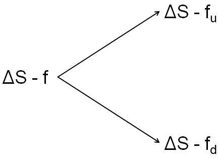
1-step binomial model
The no-arbitrage argument plays a central role for the binomial model. It states that option prices are priced in such a way that there is no arbitrage possibility left. This means that options are valued relatively with their underlying. As a result, a share and option combination can be constructed such that the portfolio value is the same in any future states. Because, this combination has the same value in any future state, it has to be risk free and thus earn the risk free rate.
Binomial model ingredients
In order to make a risk free portfolio, the delta needs to be determined. This will make sure that any change in the shares is offset by a similar but opposite change in value in the option.

Now that the portfolio is risk free, it will just earn the risk free rate over time.

This can be rearranged such that the option value today can be calculated. The following equations state that the option price today equals the expected value of the options, using the risk neutral probabilities, discounted to today by the risk free rate.


This reasoning can further be expanded into multiple time steps: 2,3,4 or more time steps.
Binomial model and Brownian motion
The previous model can further be linked to an assumed underlying stochastic process of the underlying.

When the previous assumption is made, the following variables needed in the binomial model can be calculated as follows. From these, a tree can be constructed which provides the option value.


Binomial model and american option valuation
The previous outlined steps can be used to value european style options. In order to value american options, first construct a tree to value a european option. Then check at every node whether the intrinsic value is larger than the calculated value. Replace it, if this is the case and compute the values at all previous nodes as shown in the Excel file.
Summary
The binomial model can be used to value options. These can both be european or american style and even have a more complex nature. The key idea behind the model is the no-arbitrage conditions which guarantees that options are priced correctly relatively to their underlying.
Binomial model Excel implementation
Need to have more insights? Download our free excel file: Binomial model.