
Interest rate compounding
Interest rate compounding is probably the most important topic any depositor or investor should master. A lack of knowledge in this area will definitely lead to mistakes that cause you to make financial mistakes or that make you choose less profitable investment opportunities. These are mistakes that can easily be avoided. Important aspects to which you should always devote a sufficient amount of attention are the time horizon over which interest is received and the particular compounding frequency.
Basics on interest
Using the following formula we can easily demonstrate interest rate calculation for a 1 year period. B represents the starting capital, r refers to the annual interest rate, and E equals the ending value of the capital invested.

Let’s consider a simple example. Let B be equal to 1000 and r to 10%.

Given our formula, the value of capital in 1 year will be equal to 1100.
Annual compounding
Now suppose you receive an interest of 10% annually but you keep your money at the bank for 2 years. In this case the previous formula should be adjusted slightly. In particular, we add a power t which specifies the amount of time a certain amount is invested.

Of course, at the end of the first year the result will the the same as in the previous example: E=1100.

The ending value at the end of year 2 equals 1210, which exceeds 1200. This is because you earn interest on the interest received at the end of the first year: 10% on the initial 1000 and 10% on the additional 100 earned during the first year.

Periodically compounding
The second important aspect of interest rates is the frequency with which the interest is compounded. Let’s denote this compounding frequency with the variable m. The following equation includes this variable, which represents the number of times a year interest is compouned.

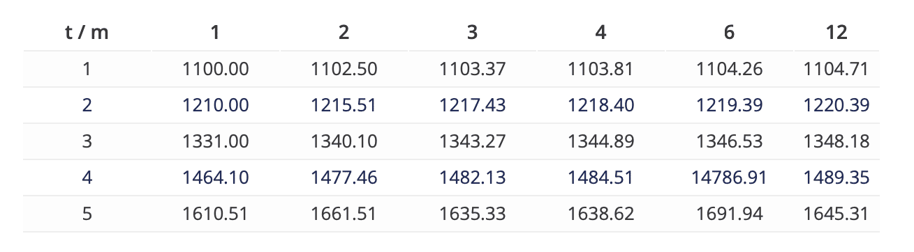
Building further on our previous example, suppose the interest rate is compounded every 6 months. In that case m equals 2. For the first year, E will be equal to 1102.50. This is higher than 1100 in the case of annual compounding. Again, this is the result of compounding, which is now performed twice a year (‘biannual’) at a rate of 10% a year instead of only once at the end of the year (‘annual’).

At the end of the second year, E equals 1215.51 instead of just 1210.

The following table further illustrates the importance of time and impact of periodically compounding. The longer the investment horizon and the more frequent interest is compounded, the higher the capital will be at the end of the investment horizon.
Continuous compounding
If we further increase m, meaning that we increase the number of compounding periods, ending capital will increase even more. Theoretically, m can be decreased to arbitrarily short intervals close to zero. In that case, interest is compounded ‘continuously’. In mathematical terms, this result means that we can represent the previous formula as the number e taken to the power of t multiplied by the interest rate r.

Applying the above formula with B equal to 1000 and an r equal to 10%

we find a terminal value of 1105.17.
Summary
Interest rate calculations should be part of the toolbox of every investor. Investment horizons and the periodacy of compounding affect the final realised wealth more than one would expect at first sight.
Interest compounding
Need to have more insights? Download our free excel file: interest compounding