Modern Portfolio Theory of Markowitz

The Modern portfolio theory (MPT) of Markowitz, also referred to as mean-variance optimization (MVO) is a statistical method that can be used to construct a mean-variance efficient portfolio of securities. Markowitz portfolio selection

The approach was introduced by Harry Markowitz in 1952 in a paper titled “Portfolio Selection”. MVO allows investors to construct a portfolio that gives investors the best risk/return trade-off available. To be apply to apply the portfolio construction approach we discuss here, you need to master some basics statistics. These statistics are explained in basic statistics.

Constructing portfolios

For simplicity, let’s start off with two companies, company A and company B. We want to invest our money in one or both of the firms by buying shares from the companies. Markowitz’s portfolio selection approach allows us to determine how we should spread our investment. For simplicity, let us assume we already did some analysis. We obtained the following set of expected returns and standard deviations for both companies’ stocks.

Now, we first define the expected return of the entire portfolio, denoted E(r_p). This is very simple, as it is just the weighted average of the expected returns of the companies’ stocks included in the portfolio.

$E(r_p) = w_A \cdot E(r_A) + w_B \cdot E(r_B)$

w_A and w_B represent the fraction of the money invested in each of the companies’ stock. These are the values we want to determine.

Next, we need to calculate the riskiness of the corresponding portfolio. This is a bit more complicated. This is because the securities are potentially correlated.

$\sigma_p^2 = w_A^2 \cdot \sigma_A^2 + w_B^2 \cdot \sigma_B^2 + 2 \cdot w_A \cdot w_B \cdot cov(r_A,r_B)$

We can rewrite the above formula to show the impact of correlation

$\sigma_p^2 = w_A^2 \cdot \sigma_A^2 + w_B^2 \cdot \sigma_B^2 + 2 \cdot w_A \cdot w_B \cdot \rho_{A,B} \cdot \sigma_A \cdot \sigma_B$

Correlation (denoted with the symbol $rho$ ) can take on values between -1 (perfect negative correlation) and +1 (perfect positive autocorrelation). Having rewritten the equation we can clearly see that the higher the correlation between stocks A and B, the higher the riskiness of the overall portfolio.

We can illustrate the effect of correlation on diversification using a simple table. Suppose we invest 50% in each of the two companies’ stock. In that case, we have all the inputs for the above equation, except for the correlation coefficient.

Now, if we vary the the correlation coefficient, we see that the standard deviation of our portfolio varies. The standard deviation is lowest when both stocks are perfectly negatively correlated ( $rho$ = -1), and highest when we have perfect positive autocorrelation ( $rho$ = 1).

Efficient frontier of portfolios

Next, we plot the relationship between the return and the riskiness of a portfolio for the actual level of autocorrelation of both stocks. Let’s assume that both stocks are negatively correlated, say $rho$ = -0.6. Rather than varying the degree of autocorrelation, we now vary the weights we invest in both stocks (i.e. $w_A$ and $w_B$ ). Thus, we plot all the possible combinations of both portfolios we can invest in.

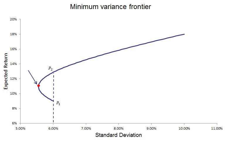
We call the above line the minimum variance frontier. It indicates the minimum variance (i.e. riskiness) that can be reached for each level of expected return.

However, there are portfolios on this minimum variance frontier that are quite unattractive. This is because we can choose another portfolio that will give us a higher return, for the same amount of risk. this is the case for all the portfolios below the global minimum variance portfolio. If we drop this ‘inefficient’ part of the frontier, what’s left is the efficient frontier or Markowitz frontier.

All the portfolios on this frontier provide the best return for a given amount of risk. All combinations above this line cannot be reached with the stocks in our portfolio. All the combinations below can be reached, but are inefficient. We also find that the efficient frontier is non-linear and that it has a slowly decreasing slope. This means that as we take on more risk, the expected return of the portfolio increases less.

As some of you might have noted, we still still haven’t answered the question of which weights w_A and w_B we should actually choose. As such, we still need to determine the optimal risky portfolio on this frontier.