
Parametric value-at-risk
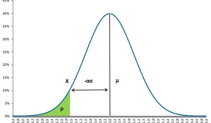
The parametric value-at-risk model is the best starting point to the get insight in the methodology. The parametric value-at-risk model is build on the normal distribution which requires an estimate of volatility (and the mean return) to indicate a portfolio’s market riskiness. In order to calculate a VaR, you first need to estimate the portfolio’s or security’s volatility, σ, the money invested in the portfolio or security, W, and if required the expected return, μ. Thereafter, the VaR can be calculated by imposing a certain probability and time horizon. Based on the normal distribution, the values of α equal 1.282, 1.645 or 2.326 when fixing the probability on 90%, 95% and 99% respectively.

Obviously, the main benefit of this model is its simplicity. Without any additional estimation, a VaR on a different time horizon and,or a different probability can directly be derived from the same information. The downside is that the assumed normal distribution may not be true which can be accommodated by assuming a t-distribution allowing for fatter tails.
Parametric value-at-risk and confidence intervals
One of the greatest benefits of this model is its capability to adjust the probability of not having a loss exceeding the VaR. This can be done using exactly the same data and applying the formula again.
Parametric value-at-risk and time
Value-at-risk measures incorporate an underlying time horizon. The calculation of a new value-at-risk measure with another time horizon can be done in 2 ways. The first way is by collecting the appropriate volatility (and return) over the new time horizon. For example, collecting both volatility and return over a 10 day period. The second approach, used the square root of time rule. This can only be applied if previous VaR measures are calculated without incorporating return. Thus by setting the return to 0 as shown below.

The new VaR measure can than quickly be calculated as:

If for example the new VaR measures is based on a 10 day period and the initial VaR on a 1 day period, the VaR_{10 days} can be calculated as:

Parametric value-at-risk and linearity
The parametric value-at-risk is most suited to measure market risk in linear derivatives: forwards, futures and swaps. They are not suited being applied to options and bonds which both show nonlinear behaviour. Value-at-risk measures based on Monte Carlo simulations or historical simulations are better suited for those.
Summary
The parametric value-at-risk models allows to calculated the probability of a loss not exceeding a certain threshold during some time period. The model is based on the normal distribution and can be easily tailored to the user’s requirements.
Parametric value-at-risk Excel implementation
Need to have more insights? Download our free excel file: value at risk.