
Mark to Market Variance Swap
The value of a variance swap is zero at initiation, but over time, the swap will either gain or lose value as realised and implied volatility diverge. At any point, the expected variance at maturity is simply the time-weighted average of the variance realised over the time since swap inception and the implied variance over the remaining time to maturity. As a consequence, the variance swap’s value becomes less and less dependent on the remaining implied volatility. On this page, we discuss how mark to market variance swap valuation can be performed using a numerical example. A spreadsheet that implements the approach is available at the bottom of this page.
Mark to market process
Let’s consider a one-year swap where three months have elapsed since inception. Marking to market requires three steps:
- First, we need to compute the expected variance at maturity (the time-weighted average of realised variance and implied variance over the remainder of the swap’s life).

where sigma² is the annualised realised volatility from initiation to valuation date squared. K²(T-t) is the annualised implied volatility from valuation date to swap maturity squared.
- Next, compute the expected payoff at swap maturity:

- Finally, we discount the expected payoff at maturity back to the valuation date.
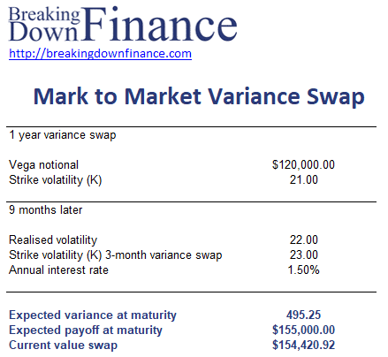
Mark to market example
To clarify the approach, we now apply the above steps to a numerical example. The following table illustrates all the necessary steps in a mark to market variance swap valuation. The spreadsheet used is available at the bottom of the page.
Summary
We discussed how to mark to market variance swaps. More details on variance swaps can be found here. Typically, variance swaps are quoted using vega notional.
Download the Excel spreadsheet
Want to have an implementation in Excel? Download the Excel file: Mark to market variance swap Example