
Quantity Theory of Money
The Quantity Theory of Money (QTM), also referred to as the classical quantity theory of money, is a very famous theory that relates the price level in an economy to the amount of money in circulation in that economy. In particular, the QTM theory argues that there is a proportionate and direct relationship between both variables. As a consequence, any increase in the money supply will not have any real effect on economic activity. Instead, increases in the money supply only increase the prices of goods and services (i.e. inflation).
On this page, we explain the Fisher’s quantity theory of money, discuss the quantity theory of money formula, and illustrate the theory using a simple example that illustrates how an increase in the money supply determines the inflation rate.
Quantity Theory of Money definition
The QMT is one of the cornerstones of financial economics. It was first formulated by Irving Fisher in the 1930s. The quantity theory of money states that when central banks increase the money supply, this increase in the amount of money in circulation will only increase prices in the long-run. It will have no effect on real variables. Thus, the quantity theory of money describes the relationship between the growth in the money supply and the inflation rate.
The Quantity theory of money formula
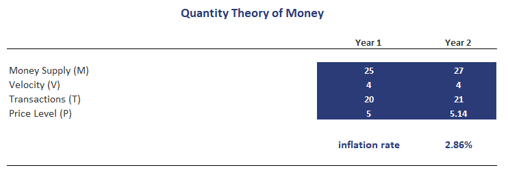
Fisher’s equation of the quantity theory of money consists of four variables; the velocity of money V, the money supply M, the price level P, and the number of transactions T

This formula is also referred to as the equation of exchange. It relates the inflation rate to the money supply in a very simple way.
Cambridge version of Quantity Theory of Money
A slightly different approach to formulating the theory is the Cambridge version of the QMT, proposed by Maynard Keynes. The difference between Fisher and Cambridge quantity theory of money is that the latter assumes that a certain fraction is of the money k is held for convenience and security. Thus, the Cambridge equation is for the QTM equals

where Md is the money demand, P is the price level and Y is economic output.
Friedman’s restatement
Related to this classical Quantity Theory of Money is Friedman’s restatement of the Quantity Theory of Money, written in 1956. The big adjustment to the QMT suggested by Friedman is that velocity is not a passive function of the quantity of money. Instead Friedman argues that when the amount of money increases, the velocity also tends to go up, and vice versa.
limitations of Quantity Theory of Money
The main limitation of the QMT is that it is based on unrealistic assumptions. In particular, the idea of full employment and that expenditure will remain stable are unrealistic. Another limitation of the QMT is that it is only tends to work in the long run, but is not very useful in the short run. Finally, it does not propose any casual relationship between the money supply and the price level, which may be related to each other.
Quantity Theory of Money example problems
Finally, we discuss some quantity theory of money example problems to get some more intuition of how to apply the equation
Summary
The QTM is a theory of how increases in the amount of money in circulation lead to higher inflation.
QTM implementation
Want to have an implementation in Excel? Download the Excel file: Quantity Theory of Money example