
Monte Carlo value-at-risk
The third approach in estimating the value-at-risk metric applies the Monte Carlo technique. In Monte Carlo value-at-risk, the simulation process is based on 2 ingredients: an underlying stock price process, and an assumed distribution. Often, the normal distribution is assumed but this is not a requirement and can in fact be any distribution. The geometric Brownian motion, as shown below, can be used as an underlying stock price. With S being equal to the price of the stock, μ equal to the stock’s return, σ equal to the stock’s volatility and Δt equal to 1 time step.

Monte Carlo value-at-risk implementation
In order to implement the stock price evolution in Excel this has to be restated as follows:

With an uncertainty parameter ε generated by a certain distribution, often just a normal distribution.

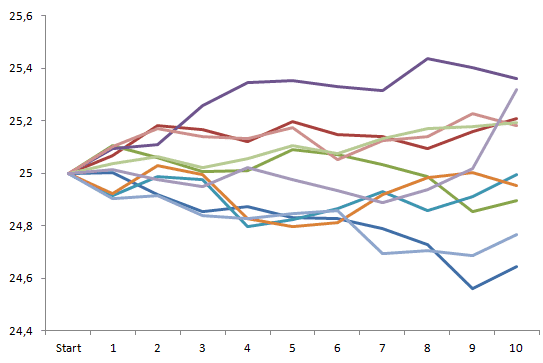
From these, multiple prices processes over a certain period (1 day, 10 days, 1 year,…) can be constructed as shown in the figure below. Thereafter, the x-period return is calculated and stored. After having stored al simulated x-day returns, the x% value-at-risk measure can be determined. This can be done through sorting the returns from small to large and selecting the appropriate percentage: 1%, 5% or 10%.
Summary
The Monte Carlo value-at-risk metric is calculated based on an underlying price process and an imposed distribution on the uncertainty parameter. It can be used to calculate the value-at-risk measure for both linear and nonlinear contracts. Moreover, it can be applied to both a single or multiple securities.
Monte Carlo value-at-risk Excel implementation
Need to have more insights? Download our free excel file: monte carlo value at risk.