Vasicek Model

The Vasicek Model or Vasicek interest rate model is a single factor interest rate model. The model allows us to model the evolution of short-term interest rates. The single factor used in the model captures market risk. The Vasicek interest rate model is extensively used to determine bond prices, model credit risk, and to price interest rate derivatives. The model was introduced by Oldřich Vašíček in 1977. Oldřich Vasicek is also famous for his work for modeling loan portfolio values as well as for the Vasicek beta adjustment.

On this page we discuss the Vasicek interest rate model, discuss the model calibration, and finally provide the Vasicek model in Excel. The Excel spreadsheet can be found at the bottom of the page.

Vasicek model

The model can be summarized in a single formula that describes a short-term interest rate’s behaviour. The Vasicek formula

$dr_t = a(b-r_t)dt + \sigma dW_t$

where Wt is a Wiener process that describes the market risk factor. First, we have the standard deviation sigma, which sets the volatility of the short-term interest rate. Next, we have the parameters a and b. These, together with sigma and the initial condition rt, describe all the dynamics in the model. But how should we interpret a and b?

The interpretation, assuming a is not negative, goes as follows:

b: the long-term mean level. All interest rate paths evolve around b
a: mean-reversion speed. It characterises the speed with which the simulated path goes back to b

Finally, there is also an important ratio we can derive from the model

$\frac{\sigma^2}{2a}$

This ratio measures the degree of long-term variance. All price paths of the interest rate will revert around the long-term mean with this degree of variance.

Cox Ingersoll Ross vs Vasicek

Looking at the model, we should note that it is a mean-reverting model. This makes sense, since interest rates cannot go up indefinitely and do not go below zero for long periods of time either. Instead, interest rates tend to revert back to certain ‘natural’ levels. This is the big contribution of the model.

The big disadvantage of the model is that interest rates can become negative. Of course, given the recent financial crisis, we learned that negative interest rates can occur more frequently than we imagined possible.

A number of other models are extensions of the Vasicek model. These include the Hull-White model and the Cox-Ingersoll-Ross model, the Black-Derman-Toy model and the Black-Karasinski model. The big difference between these models and the Vasicek model is that the extensions such as the Cox-Ingersoll-Ross model address the ‘problem’ that interest rates can turn negative under the Vasicek’s model.

Vasicek model calibration

The Vasicek calibration is an important aspect of the Vasicek interest rate model. To calibrate the model, analysts typically perform a simple ordinary least squares (OLS) regression using actual daily interest rate data. This is needed to determine a, b, and sigma in the model.

Vasicek model solution

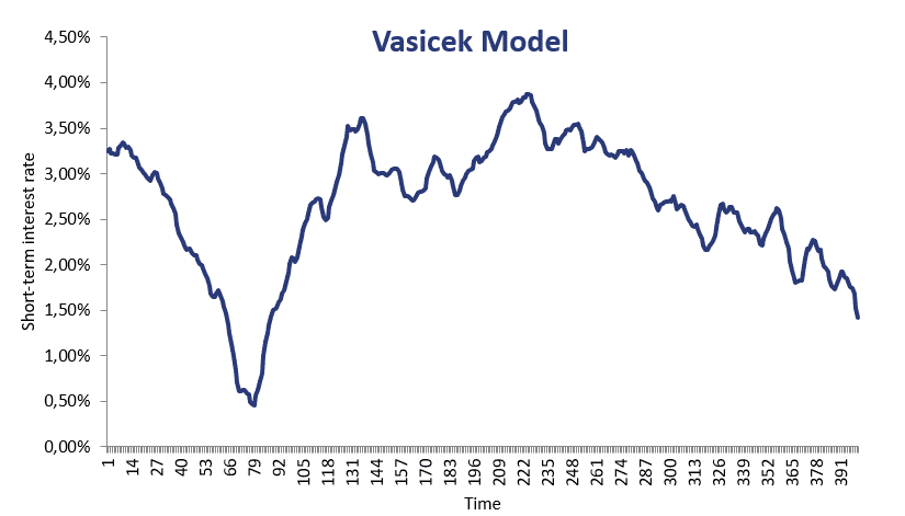
In the Excel spreadsheet at the bottom of the page we implement the necessary routines to apply the model. The Vasicek model calibration is not discussed, but can also be don using Excel’s solver features. Finally, we note that using the simulated interest rates, it is very easy to use the model to determine bond prices. The following figure illustrates how interest rates can be simulated using the model.

Summary

We discussed a short-term interest rate model that is mean-reverting.

Download the Excel spreadsheet

Want to have an implementation in Excel? Download the Excel file: Vasicek Model template