
Expansion Project Analysis
Expansion Project Analysis is used by a company’s management to evaluate capital projects. The methodology builds on the net present value (NPV) methodology. The most important step when applying project analysis is to identify the relevant cash flows. In particular, capital budgeting looks at the incremental after-tax cash flows. Once we have the cash flows, it is easy to calculate the NPV or IRR.
On this page, we discuss expansion project analysis. This is a different approach than the replacement project analysis approach we discuss elsewhere. Here, we discuss the three types of cash flows that have to be determined to apply an expansion project analysis and illustrate the approach using an Excel spreadsheet example.
Expansion project analysis formula
There are three cash flows we need to determine. The first kind of cash flow is the initial investment outlay. The initial investment outlay consists of two components

The first component is the fixed capital investment (FCInv). This consists of the price paid for the machinery, including the shipping and installation. The second component is the investment in net working capital (NWCInv). The formula for the net working capital investment equals

The investment in NWC consists of the additional inventories required, increases in accounts receivable, and it decreases with increases in accounts payable and accruals. If NWCInv is positive (negative), additional financing is required (available). At the termination of the project, these funds become available again.
Next, we need to calculate the second kind of cash flow, the after-tax operating cash flows (CF). The after-tax operating cash flow formula equals

where S is sales, C is cash operating costs, D is depreciation expense, and T is the marginal tax rate. Depreciation is subtracted because it lower the tax bill. We add it again afterwards because it is a non-cash expense.
Finally, we have to calculate the terminal year after tax non-operating cash flows (TNOCF). The terminal year after-tax non-operating cash flow formula looks as follows

where Sal is the pre-tax cash proceeds from the sale of the machine and B is the book value of the machine when sold
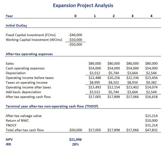
Expansion project analysis example
Next, let’s have a look at a numerical example. The following table shows the results of an implementation of the methodology using an Excel spreadsheet. The spreadsheet can be downloaded at the bottom of the page.
Summary
We discussed expansion project analysis, a capital budgeting approach to evaluate the attractiveness of capital projects. An extension of this approach is expansion project analysis.
Download the Excel spreadsheet
Want to have an implementation in Excel? Download the Excel file: Expansion Project Analysis