
Value Averaging (VA)
Value averaging, or value average investing, is an investment technique proposed by Michael Edleson. It’s a mechanical investment approach that helps investors to decide when and how much money to allocate to an investment portfolio. The value averaging calculator in the spreadsheet below allows you to calculate the number of shares that should be bought to meet a predetermined (interim) target value. Value averaging is closely related to dollar cost averaging (DCA).
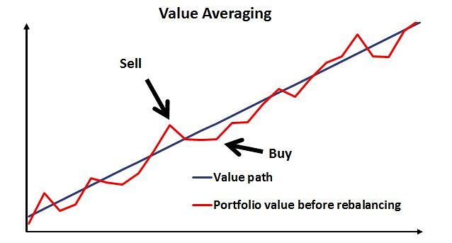
Intuitively, the idea is to invest money in such a way that the value of our investments meets a pre-determined target value at every point in time. To succeed, we will need to invest more in some periods compared to others. In addition, if our portfolio has gone up considerably, we might even have to sell some of our securities.
Hence, value averaging also provides sell signals. When properly applied, value averaging should help us to ‘buy low, sell high‘. Research suggests that value averaging works better than another often cited technique called Dollar-cost Averaging (DCA).
Below we provide a spreadsheet in Microsoft Excel to implement a value averaging investing approach.
Value averaging formula
The value averaging approach requires us to set both the target value that we wish to obtain, as well as the expected growth rate of our investment. The expected growth rate of the investment is the annual return we expect the investment to generate.
Value averaging is different from dollar-cost averaging. In the case of dollar-cost averaging, we define the periodic investment (e.g. US$ 500 every quarter), and invest that money no matter how stock markets evolve. This will ensure that we buy fewer stocks when stock prices are high, and more stocks when stock prices are low.
By also taking into consideration the expected growth rate of the investment, we can take into account periods in which stock prices go up a lot. In that case, it’s probably better to sell some of our holdings, instead of adding more money to the existing position. If the return exceeds our expected growth rate over a certain period, we should sell (high) some of our position. Instead, if the actual return is less than expected, we should add more to the portfolio to make sure we reach our target. In that case, we will be buying low.
Central to value averaging is the so-called Value Path. Theis value path describes our investment’s target value we wish to achieve at different points in time. Then, we just make the necessary investment (or divestment) so that the value of our holdings equals the interim target value.
Let’s describe the value path in mathematical terms. The value path (Vt) equals

where
- t: number of time periods (in months, quarters, years,…),
- C: target initial contribution at time t,
- r: expected rate of growth per period of investment (monthly, quarterly, or annual return),
- g: expected rate of growth per period of the contribution (monthly, quarterly, or annual return),
- R: average rate of growth of investment and contribution (monthly, quarterly, or annual return)
For simplicity, we’ve assumed that

In other words, R equals the average of the expected growth rates of the investment and the contribution.
Numerical example value averaging
Let’s discuss two common ways in which the above formula can be applied in our investment approach. First, it could be that we have a specific goal in mind. For example, we want to have US$ 200,000 by the time we retire (e.g. in 20 years). In that case we have the target value (Vt) in mind and we can determine the required (initial) annual contribution C. Let’s assume we invest Mathematically,

Alternatively, we might not have a particular goal in mind. Instead, we have an idea of how much money we can allocate to our portfolio at every point in time. Then, we can construct the Value path to see how our portfolio will evolve over time. In the Excel spreadsheet below, we implement the value averaging approach just described.
There is one thing we should definitely keep in mind when using value averaging to manage a portfolio. The outcome of value averaging is highly dependent on our estimate of the expected growth rate of the investment. As such, it’s better to use a conservative (i.e. lower) estimate. Especially since we want to avoid ending up below the target value. Also, by plugging in conservative figures we might reach our goal earlier.
Value averaging – how many stocks to buy
The above discussed approach is not that easy to implement in practice. Value averaging gives you a good idea of how much you need to invest to obtain a certain target value. However, the way we described it above, it does not give a straightforward answer to the question most investors struggle with:
how many stocks to buy?
In the spreadsheet, we provide a simple example to determine the number of stocks you should buy (or sell) to stay on the value path you set out.
Summary
Value averaging is a useful tool when you want to add to an investment portfolio periodically. In particular, it suggests the number of stocks you should buy or sell.
Value Averaging Excel implementation
Want to learn more about value averaging? Download our free excel file: Value Averaging.